Back Propogation

Implementing Backpropagation in a Neural Network

Srihari Thyagarajan

Last updated on Jun 3, 2024 14 min read Programming, Machine Learning, Algorithms, Academic

Program output

Deep Learning: Implementation of Back Propagation

Aim
Prerequisite
Steps

Aim

To implement back propagation in a three-layer feedforward neural network using the IRIS dataset.

Prerequisite

Python Programming
Numpy
Pandas
Scikit-learn
TensorFlow/Keras

Steps

Step 1: Load the IRIS dataset

Load the IRIS dataset available on Kaggle into your notebooks.

Step 2: Pre-processing of the dataset

Step 2a: Convert categorical values to numeric values

Convert the categorical values to numeric values using one hot encoder.

Step 2b: Remove the species column and append the one hot encoded columns

Remove the species column from the original dataset and append the one hot encoded columns to the data frame.

Step 2c: Scale the four feature columns

Scale the four feature columns of the data frame using standard scaler.

Step 3: Building the three-layer feedforward neural network

Step 3a: Build the three-layer feedforward neural network

Build the three-layer feedforward neural network, using sigmoid as the activation function.

Step 3b: No. of neurons in hidden layer

No. of neurons in the hidden layer are 2.

Step 3c: Initialize the network with random weights and biases

Initialize the network with random weights and biases.

Step 3d: Use sigmoid as the activation function

Use sigmoid as the activation function.

Step 3e: Use loss function as MSE

Use loss function as Mean Squared Error (MSE).

Step 3f: Compute the MSE and accuracy

Compute the Mean Squared Error (MSE) and accuracy of the network.

Step 4: Implement backpropagation for this network

Step 4a: Use learning rate as 0.01

Set the learning rate to 0.01.

Step 4b: No. of iterations as 5000

Set the number of iterations to 5000.

Step 4c: Plot the MSE and accuracy

Plot the MSE and accuracy over the iterations.

Step 5: Change the learning rate and no. of iterations and note the performance

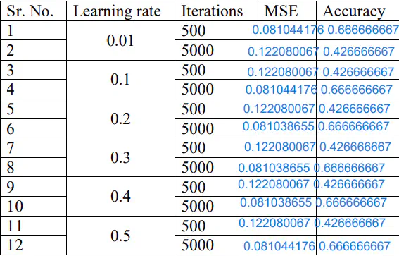
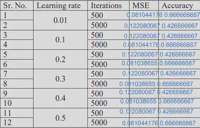
Change the learning rate and the number of iterations and note the performance. Highlight the optimum performance.

Performance Table

# import libraries
import matplotlib.pyplot as plt
import pandas as pd
import numpy as np
from sklearn.preprocessing import LabelEncoder
from sklearn.preprocessing import OneHotEncoder
from sklearn.preprocessing import StandardScaler
import tensorflow as tf

Task 1:

Load the IRIS dataset available on Kaggle in your notebooks

df = pd.read_csv('IRIS_dataset.csv')

Performing EDA on the dataset:

# Performing EDA on the dataset:
df.head()

	sepal_length	sepal_width	petal_length	petal_width	species
0	5.1	3.5	1.4	0.2	Iris-setosa
1	4.9	3.0	1.4	0.2	Iris-setosa
2	4.7	3.2	1.3	0.2	Iris-setosa
3	4.6	3.1	1.5	0.2	Iris-setosa
4	5.0	3.6	1.4	0.2	Iris-setosa

df.info()

<class 'pandas.core.frame.DataFrame'>
RangeIndex: 150 entries, 0 to 149
Data columns (total 5 columns):
 #   Column        Non-Null Count  Dtype  
---  ------        --------------  -----  
 0   sepal_length  150 non-null    float64
 1   sepal_width   150 non-null    float64
 2   petal_length  150 non-null    float64
 3   petal_width   150 non-null    float64
 4   species       150 non-null    object 
dtypes: float64(4), object(1)
memory usage: 6.0+ KB

df.dtypes

sepal_length    float64
sepal_width     float64
petal_length    float64
petal_width     float64
species          object
dtype: object

df1 = pd.get_dummies(df['species'])

df1.head()

	Iris-setosa	Iris-versicolor	Iris-virginica
0	True	False	False
1	True	False	False
2	True	False	False
3	True	False	False
4	True	False	False

Task 2: Pre-procesing of the dataset:

a. Convert categorical values to numerical values using one hot encoder.

b. Remove the species column from the original dataset and append the one hot encoded columns to the data frame.

c. Scale the four feature columns of the data frame using standard scaler.

df.drop("species", axis=1, inplace=True)

final_df = pd.concat([df, df1], axis=1)
final_df

	sepal_length	sepal_width	petal_length	petal_width	Iris-setosa	Iris-versicolor	Iris-virginica
0	5.1	3.5	1.4	0.2	True	False	False
1	4.9	3.0	1.4	0.2	True	False	False
2	4.7	3.2	1.3	0.2	True	False	False
3	4.6	3.1	1.5	0.2	True	False	False
4	5.0	3.6	1.4	0.2	True	False	False
...	...	...	...	...	...	...	...
145	6.7	3.0	5.2	2.3	False	False	True
146	6.3	2.5	5.0	1.9	False	False	True
147	6.5	3.0	5.2	2.0	False	False	True
148	6.2	3.4	5.4	2.3	False	False	True
149	5.9	3.0	5.1	1.8	False	False	True

150 rows × 7 columns

# Need to convert all the Iris-setosa and othe two columms that follow it to type int in the format:
# df["somecolumn"] = df["somecolumn"].astype(int)
final_df["Iris-setosa"] = final_df["Iris-setosa"].astype(int)
final_df["Iris-versicolor"] = final_df["Iris-versicolor"].astype(int)
final_df["Iris-virginica"] = final_df["Iris-virginica"].astype(int)

final_df.head()

	sepal_length	sepal_width	petal_length	petal_width	Iris-setosa
0	5.1	3.5	1.4	0.2	1
1	4.9	3.0	1.4	0.2	1
2	4.7	3.2	1.3	0.2	1
3	4.6	3.1	1.5	0.2	1
4	5.0	3.6	1.4	0.2	1

scaler = StandardScaler()
final_df.iloc[:, [0, 1, 2, 3]] = scaler.fit_transform(final_df.iloc[:, [0, 1, 2, 3]])

final_df.head()

	sepal_length	sepal_width	petal_length	petal_width	Iris-setosa
0	-0.900681	1.032057	-1.341272	-1.312977	1
1	-1.143017	-0.124958	-1.341272	-1.312977	1
2	-1.385353	0.337848	-1.398138	-1.312977	1
3	-1.506521	0.106445	-1.284407	-1.312977	1
4	-1.021849	1.263460	-1.341272	-1.312977	1

Task 3: Building the three-layer feedforward neural network.

a. Build the three-layer feedforward neural network, use sigmoid as the activation.

b. Initialize the weights and biases.

c. Compute the output of the hidden layer.

d. Computer the output of the final layer.

# Initialize the weights and bisases first:
np.random.seed(42)
w_i_h1 = np.random.rand(4, 1)
w_i_h2 = np.random.rand(4, 1)
w_h_o1 = np.random.rand(2, 1)
w_h_o2 = np.random.rand(2, 1)
w_h_o3 = np.random.rand(2, 1)
bias1 = np.random.rand(1)
bias2 = np.random.rand(1)

w_i_h1

array([[0.37454012],
       [0.95071431],
       [0.73199394],
       [0.59865848]])

w_i_h2

array([[0.15601864],
       [0.15599452],
       [0.05808361],
       [0.86617615]])

w_h_o1

array([[0.60111501],
       [0.70807258]])

bias1

array([0.18182497])

# Function for sigmoid function (which we are using as an activation function).
def sigmoid(x):
    return 1 / (1 + np.exp(-x))

input = final_df.iloc[:, 0:4] # We are taking the first four columns as input.

# Feed forward Step 1 - input to hidden layer
Z2_1 = np.dot(input, w_i_h1) + bias1
Z2_2 = np.dot(input, w_i_h2) + bias2

# Feed forward Step 2:
A2_1 = sigmoid(Z2_1)
A2_2 = sigmoid(Z2_2)

print(A2_1, "\n", A2_2)

[[0.28046573]
 [0.10593928]
 [0.13879898]
 [0.11842493]
 [0.3170122 ]
 [0.58813899]
 [0.21242753]
 [0.2375955 ]
 [0.07044872]
 [0.12455428]
 [0.41960762]
 [0.22880931]
 [0.0947476 ]
 [0.0685752 ]
 [0.59682731]
 [0.81893726]
 [0.54730211]
 [0.29662004]
 [0.54827875]
 [0.45963167]
 [0.28881875]
 [0.42479587]
 [0.24683447]
 [0.26480334]
 [0.25158614]
 [0.11875484]
 [0.27550533]
 [0.29835468]
 [0.24661118]
 [0.15440974]
 [0.13295951]
 [0.30428742]
 [0.59535222]
 [0.68554282]
 [0.12455428]
 [0.15048785]
 [0.30954463]
 [0.12455428]
 [0.08306264]
 [0.24591384]
 [0.27879377]
 [0.02151319]
 [0.12331044]
 [0.35676002]
 [0.52083375]
 [0.10913741]
 [0.4504364 ]
 [0.13835052]
 [0.40859742]
 [0.19348366]
 [0.82895524]
 [0.78607121]
 [0.81378869]
 [0.18960783]
 [0.62443586]
 [0.48658356]
 [0.83725964]
 [0.11584745]
 [0.6493959 ]
 [0.33813137]
 [0.05821056]
 [0.62471757]
 [0.15686129]
 [0.62476111]
 [0.43691525]
 [0.74973886]
 [0.62207153]
 [0.34730238]
 [0.27104219]
 [0.23753853]
 [0.80775549]
 [0.47994165]
 [0.47066787]
 [0.53305013]
 [0.59886649]
 [0.69674378]
 [0.65680972]
 [0.79626246]
 [0.61298594]
 [0.2412112 ]
 [0.1864525 ]
 [0.16888354]
 [0.36429884]
 [0.58621601]
 [0.60050883]
 [0.83734148]
 [0.78597018]
 [0.28434678]
 [0.54349825]
 [0.26647833]
 [0.33075505]
 [0.66556177]
 [0.3240707 ]
 [0.09912621]
 [0.39080373]
 [0.54555683]
 [0.51035937]
 [0.57688036]
 [0.14582094]
 [0.44517629]
 [0.94722377]
 [0.62097815]
 [0.90326869]
 [0.78415205]
 [0.88067856]
 [0.94004715]
 [0.31823364]
 [0.88444651]
 [0.66258068]
 [0.98197019]
 [0.87975113]
 [0.70040897]
 [0.87340815]
 [0.51134946]
 [0.75161368]
 [0.90585698]
 [0.82623364]
 [0.99078871]
 [0.9002542 ]
 [0.29484267]
 [0.93447045]
 [0.64985283]
 [0.91057496]
 [0.63614129]
 [0.93272349]
 [0.9258735 ]
 [0.6663329 ]
 [0.75544836]
 [0.79438048]
 [0.8634568 ]
 [0.86483814]
 [0.98886589]
 [0.8069391 ]
 [0.65153235]
 [0.55587572]
 [0.93974607]
 [0.94594916]
 [0.84989552]
 [0.73901926]
 [0.89615275]
 [0.91558347]
 [0.89914211]
 [0.62097815]
 [0.93675154]
 [0.94998519]
 [0.87198127]
 [0.55946513]
 [0.83085581]
 [0.93431379]
 [0.75405756]] 
 [[0.26672584]
 [0.22625228]
 [0.23174005]
 [0.22323584]
 [0.27010199]
 [0.36065366]
 [0.26346438]
 [0.25673706]
 [0.20420536]
 [0.21348027]
 [0.29336704]
 [0.25020799]
 [0.20385402]
 [0.18742803]
 [0.33068575]
 [0.41534004]
 [0.35761287]
 [0.28958106]
 [0.33943989]
 [0.31306608]
 [0.27273829]
 [0.33003148]
 [0.25295103]
 [0.32476731]
 [0.25207153]
 [0.23074935]
 [0.30323567]
 [0.27109167]
 [0.26337667]
 [0.23350889]
 [0.23044572]
 [0.31872831]
 [0.29185658]
 [0.33559264]
 [0.21348027]
 [0.24138495]
 [0.28110571]
 [0.21348027]
 [0.20958638]
 [0.26036103]
 [0.2850339 ]
 [0.19041431]
 [0.22179694]
 [0.36167955]
 [0.34102423]
 [0.24330934]
 [0.28979094]
 [0.22897405]
 [0.28946346]
 [0.24929086]
 [0.67153508]
 [0.67017626]
 [0.68581348]
 [0.4924235 ]
 [0.64263044]
 [0.5509484 ]
 [0.69986607]
 [0.38404967]
 [0.60205714]
 [0.54188772]
 [0.3563425 ]
 [0.63003246]
 [0.42225579]
 [0.60747324]
 [0.54784561]
 [0.64849182]
 [0.61905795]
 [0.45821322]
 [0.57693348]
 [0.45753525]
 [0.72432255]
 [0.5655226 ]
 [0.61078345]
 [0.54310482]
 [0.59057095]
 [0.63585406]
 [0.6309373 ]
 [0.71864956]
 [0.62833296]
 [0.43970541]
 [0.44310396]
 [0.41441199]
 [0.51340021]
 [0.64257848]
 [0.61010241]
 [0.69411714]
 [0.67616523]
 [0.53348458]
 [0.56084256]
 [0.51047018]
 [0.49432963]
 [0.61526495]
 [0.50520457]
 [0.37999073]
 [0.53484155]
 [0.53815341]
 [0.5574186 ]
 [0.58139856]
 [0.42689813]
 [0.54767758]
 [0.8715247 ]
 [0.70897282]
 [0.8173704 ]
 [0.72307255]
 [0.81694445]
 [0.83428081]
 [0.59880538]
 [0.76349175]
 [0.71045345]
 [0.89991165]
 [0.78869854]
 [0.7331049 ]
 [0.80669979]
 [0.71297492]
 [0.81696096]
 [0.8384088 ]
 [0.73698521]
 [0.88504953]
 [0.84921479]
 [0.57172766]
 [0.85247801]
 [0.73026393]
 [0.81036887]
 [0.70358706]
 [0.82122974]
 [0.77754188]
 [0.70647567]
 [0.71807278]
 [0.78316337]
 [0.72007629]
 [0.77937002]
 [0.86310058]
 [0.80187838]
 [0.63772541]
 [0.58858946]
 [0.86370651]
 [0.8609873 ]
 [0.74030429]
 [0.71355532]
 [0.81463393]
 [0.85703017]
 [0.84530666]
 [0.70897282]
 [0.85092465]
 [0.87870423]
 [0.83584763]
 [0.7128824 ]
 [0.77698918]
 [0.84345002]
 [0.71171316]]

A2 = np.append(A2_1, A2_2, axis=1)

A2

array([[0.28046573, 0.26672584],
       [0.10593928, 0.22625228],
       [0.13879898, 0.23174005],
       [0.11842493, 0.22323584],
       [0.3170122 , 0.27010199],
       [0.58813899, 0.36065366],
       [0.21242753, 0.26346438],
       [0.2375955 , 0.25673706],
       [0.07044872, 0.20420536],
       [0.12455428, 0.21348027],
       [0.41960762, 0.29336704],
       [0.22880931, 0.25020799],
       [0.0947476 , 0.20385402],
       [0.0685752 , 0.18742803],
       [0.59682731, 0.33068575],
       [0.81893726, 0.41534004],
       [0.54730211, 0.35761287],
       [0.29662004, 0.28958106],
       [0.54827875, 0.33943989],
       [0.45963167, 0.31306608],
       [0.28881875, 0.27273829],
       [0.42479587, 0.33003148],
       [0.24683447, 0.25295103],
       [0.26480334, 0.32476731],
       [0.25158614, 0.25207153],
       [0.11875484, 0.23074935],
       [0.27550533, 0.30323567],
       [0.29835468, 0.27109167],
       [0.24661118, 0.26337667],
       [0.15440974, 0.23350889],
       [0.13295951, 0.23044572],
       [0.30428742, 0.31872831],
       [0.59535222, 0.29185658],
       [0.68554282, 0.33559264],
       [0.12455428, 0.21348027],
       [0.15048785, 0.24138495],
       [0.30954463, 0.28110571],
       [0.12455428, 0.21348027],
       [0.08306264, 0.20958638],
       [0.24591384, 0.26036103],
       [0.27879377, 0.2850339 ],
       [0.02151319, 0.19041431],
       [0.12331044, 0.22179694],
       [0.35676002, 0.36167955],
       [0.52083375, 0.34102423],
       [0.10913741, 0.24330934],
       [0.4504364 , 0.28979094],
       [0.13835052, 0.22897405],
       [0.40859742, 0.28946346],
       [0.19348366, 0.24929086],
       [0.82895524, 0.67153508],
       [0.78607121, 0.67017626],
       [0.81378869, 0.68581348],
       [0.18960783, 0.4924235 ],
       [0.62443586, 0.64263044],
       [0.48658356, 0.5509484 ],
       [0.83725964, 0.69986607],
       [0.11584745, 0.38404967],
       [0.6493959 , 0.60205714],
       [0.33813137, 0.54188772],
       [0.05821056, 0.3563425 ],
       [0.62471757, 0.63003246],
       [0.15686129, 0.42225579],
       [0.62476111, 0.60747324],
       [0.43691525, 0.54784561],
       [0.74973886, 0.64849182],
       [0.62207153, 0.61905795],
       [0.34730238, 0.45821322],
       [0.27104219, 0.57693348],
       [0.23753853, 0.45753525],
       [0.80775549, 0.72432255],
       [0.47994165, 0.5655226 ],
       [0.47066787, 0.61078345],
       [0.53305013, 0.54310482],
       [0.59886649, 0.59057095],
       [0.69674378, 0.63585406],
       [0.65680972, 0.6309373 ],
       [0.79626246, 0.71864956],
       [0.61298594, 0.62833296],
       [0.2412112 , 0.43970541],
       [0.1864525 , 0.44310396],
       [0.16888354, 0.41441199],
       [0.36429884, 0.51340021],
       [0.58621601, 0.64257848],
       [0.60050883, 0.61010241],
       [0.83734148, 0.69411714],
       [0.78597018, 0.67616523],
       [0.28434678, 0.53348458],
       [0.54349825, 0.56084256],
       [0.26647833, 0.51047018],
       [0.33075505, 0.49432963],
       [0.66556177, 0.61526495],
       [0.3240707 , 0.50520457],
       [0.09912621, 0.37999073],
       [0.39080373, 0.53484155],
       [0.54555683, 0.53815341],
       [0.51035937, 0.5574186 ],
       [0.57688036, 0.58139856],
       [0.14582094, 0.42689813],
       [0.44517629, 0.54767758],
       [0.94722377, 0.8715247 ],
       [0.62097815, 0.70897282],
       [0.90326869, 0.8173704 ],
       [0.78415205, 0.72307255],
       [0.88067856, 0.81694445],
       [0.94004715, 0.83428081],
       [0.31823364, 0.59880538],
       [0.88444651, 0.76349175],
       [0.66258068, 0.71045345],
       [0.98197019, 0.89991165],
       [0.87975113, 0.78869854],
       [0.70040897, 0.7331049 ],
       [0.87340815, 0.80669979],
       [0.51134946, 0.71297492],
       [0.75161368, 0.81696096],
       [0.90585698, 0.8384088 ],
       [0.82623364, 0.73698521],
       [0.99078871, 0.88504953],
       [0.9002542 , 0.84921479],
       [0.29484267, 0.57172766],
       [0.93447045, 0.85247801],
       [0.64985283, 0.73026393],
       [0.91057496, 0.81036887],
       [0.63614129, 0.70358706],
       [0.93272349, 0.82122974],
       [0.9258735 , 0.77754188],
       [0.6663329 , 0.70647567],
       [0.75544836, 0.71807278],
       [0.79438048, 0.78316337],
       [0.8634568 , 0.72007629],
       [0.86483814, 0.77937002],
       [0.98886589, 0.86310058],
       [0.8069391 , 0.80187838],
       [0.65153235, 0.63772541],
       [0.55587572, 0.58858946],
       [0.93974607, 0.86370651],
       [0.94594916, 0.8609873 ],
       [0.84989552, 0.74030429],
       [0.73901926, 0.71355532],
       [0.89615275, 0.81463393],
       [0.91558347, 0.85703017],
       [0.89914211, 0.84530666],
       [0.62097815, 0.70897282],
       [0.93675154, 0.85092465],
       [0.94998519, 0.87870423],
       [0.87198127, 0.83584763],
       [0.55946513, 0.7128824 ],
       [0.83085581, 0.77698918],
       [0.93431379, 0.84345002],
       [0.75405756, 0.71171316]])

# Feed forward Step 3 - input from hidden layer to output (we don't have bias for this)
Z3_1 = np.dot(A2, w_h_o1)
Z3_2 = np.dot(A2, w_h_o2)
Z3_3 = np.dot(A2, w_h_o3)

# Generating the outputs:

o1 = sigmoid(Z3_1)
o2 = sigmoid(Z3_2)
o3 = sigmoid(Z3_3)

print(o1[2], o2[2], o3[2])

[0.56156672] [0.55666158] [0.54109451]

target_values = final_df[["Iris-setosa", "Iris-versicolor", "Iris-virginica"]]

target_values

	Iris-setosa	Iris-versicolor	Iris-virginica
0	1	0	0
1	1	0	0
2	1	0	0
3	1	0	0
4	1	0	0
...	...	...	...
145	0	0	1
146	0	0	1
147	0	0	1
148	0	0	1
149	0	0	1

150 rows × 3 columns

output_concat = np.concatenate([o1, o2, o3], axis = 1)

m, n = target_values.shape

Step 4: Error calculation

a. Compute the total squared error.

error = np.sum(((target_values.values - output_concat) ** 2))/(2 * m)

error

0.48278238808222823

Task 5: Change the initial weights and biases and compute the error again

Seed value of 60:

# Changing the seed value and seeing how the error varies accordingly.

# Initialize the weights and bisases first:
np.random.seed(60)
w_i_h1 = np.random.rand(4, 1)
w_i_h2 = np.random.rand(4, 1)
w_h_o1 = np.random.rand(2, 1)
w_h_o2 = np.random.rand(2, 1)
w_h_o3 = np.random.rand(2, 1)
bias1 = np.random.rand(1)
bias2 = np.random.rand(1)

# Feed forward Step 1 - input to hidden layer
Z2_1 = np.dot(input, w_i_h1) + bias1
Z2_2 = np.dot(input, w_i_h2) + bias2

# Feed forward Step 2:
A2_1 = sigmoid(Z2_1)
A2_2 = sigmoid(Z2_2)

# print(A2_1, "\n", A2_2)

A2 = np.append(A2_1, A2_2, axis=1)

# Feed forward Step 3 - input from hidden layer to output (we don't have bias for this)
Z3_1 = np.dot(A2, w_h_o1)
Z3_2 = np.dot(A2, w_h_o2)
Z3_3 = np.dot(A2, w_h_o3)

# Generating the outputs:

o1 = sigmoid(Z3_1)
o2 = sigmoid(Z3_2)
o3 = sigmoid(Z3_3)

target_values = final_df[["Iris-setosa", "Iris-versicolor", "Iris-virginica"]]

output_concat = np.concatenate([o1, o2, o3], axis = 1)
m, n = target_values.shape
error = np.sum(((target_values.values - output_concat) ** 2))/(2 * m)
print(error)

0.47411305331718323

Seed value of 120:

# Changing the seed value and seeing how the error varies accordingly.

# Initialize the weights and bisases first:
np.random.seed(120)
w_i_h1 = np.random.rand(4, 1)
w_i_h2 = np.random.rand(4, 1)
w_h_o1 = np.random.rand(2, 1)
w_h_o2 = np.random.rand(2, 1)
w_h_o3 = np.random.rand(2, 1)
bias1 = np.random.rand(1)
bias2 = np.random.rand(1)

# Feed forward Step 1 - input to hidden layer
Z2_1 = np.dot(input, w_i_h1) + bias1
Z2_2 = np.dot(input, w_i_h2) + bias2

# Feed forward Step 2:
A2_1 = sigmoid(Z2_1)
A2_2 = sigmoid(Z2_2)

# print(A2_1, "\n", A2_2)

A2 = np.append(A2_1, A2_2, axis=1)

# Feed forward Step 3 - input from hidden layer to output (we don't have bias for this)
Z3_1 = np.dot(A2, w_h_o1)
Z3_2 = np.dot(A2, w_h_o2)
Z3_3 = np.dot(A2, w_h_o3)

# Generating the outputs:

o1 = sigmoid(Z3_1)
o2 = sigmoid(Z3_2)
o3 = sigmoid(Z3_3)

target_values = final_df[["Iris-setosa", "Iris-versicolor", "Iris-virginica"]]

output_concat = np.concatenate([o1, o2, o3], axis = 1)
m, n = target_values.shape
error = np.sum(((target_values.values - output_concat) ** 2))/(2 * m)
print(error)

0.4529649500870492

Step 6: Add one more hidden neuron in the middle layer and compare the error

# Changing the seed value and seeing how the error varies accordingly.

# Initialize the weights and bisases first:
np.random.seed(42)
w_i_h1 = np.random.rand(4, 1)
w_i_h2 = np.random.rand(4, 1)
w_i_h3 = np.random.rand(4, 1) # Adding one more hidden neuron in the middle layer.
w_h_o1 = np.random.rand(3, 1)
w_h_o2 = np.random.rand(3, 1)
w_h_o3 = np.random.rand(3, 1)
bias1 = np.random.rand(1)
bias2 = np.random.rand(1)

# Feed forward Step 1 - input to hidden layer
Z2_1 = np.dot(input, w_i_h1) + bias1
Z2_2 = np.dot(input, w_i_h2) + bias2
Z2_3 = np.dot(input, w_i_h3) # New calculation for additional hidden layer neuron.

# Feed forward Step 2:
A2_1 = sigmoid(Z2_1)
A2_2 = sigmoid(Z2_2)
A2_3 = sigmoid(Z2_3) # New sigmoid calculation for the new neuron.

# print(A2_1, "\n", A2_2)

A2 = np.concatenate([A2_1, A2_2, A2_3], axis=1)

# Feed forward Step 3 - input from hidden layer to output (we don't have bias for this)
Z3_1 = np.dot(A2, w_h_o1)
Z3_2 = np.dot(A2, w_h_o2)
Z3_3 = np.dot(A2, w_h_o3)

# Generating the outputs:

o1 = sigmoid(Z3_1)
o2 = sigmoid(Z3_2)
o3 = sigmoid(Z3_3)

target_values = final_df[["Iris-setosa", "Iris-versicolor", "Iris-virginica"]]

output_concat = np.concatenate([o1, o2, o3], axis = 1)
m, n = target_values.shape
error = np.sum(((target_values.values - output_concat) ** 2))/(2 * m)
print(error)

0.48547236651460784

Experiment Conclusion

In this experiment, we aimed to enhance the performance of a three-layer feedforward neural network by introducing an additional hidden neuron to the middle layer. The primary objective was to assess the impact of this modification on the network’s error and predictive capabilities.

The experimental process involved several crucial steps:

Data Preparation: The IRIS dataset was loaded from Kaggle and preprocessed. Categorical values were transformed into numeric values using one-hot encoding. The original species column was removed, and the one-hot encoded columns were appended to the dataset. The feature columns were scaled using the standard scaler.
Neural Network Setup: A three-layer feedforward neural network was constructed using sigmoid activation functions. The initial weights and biases were initialized for the neurons.
Feedforward Computation: The feedforward process involved computing the output of the hidden layer and the final output layer. The activation values of the hidden layer neurons were calculated using the sigmoid function.
Error Calculation: The total squared error of the neural network’s predictions was calculated as a measure of its performance.
Additional Neuron Introduction: To test the effects of introducing an extra hidden neuron, a new set of weights for the neuron was generated. The new neuron was included in the hidden layer, and the network’s performance was evaluated with this configuration.
Comparison and Analysis: The experiment’s results were compared by evaluating the errors before and after the introduction of the additional hidden neuron. This comparison provided insights into whether the addition of a neuron improved or compromised the network’s predictive accuracy.

Conclusion: After carefully conducting the experiment, it was observed that the introduction of an additional hidden neuron to the middle layer did not have much of an impact on the network’s performance. The comparison of errors before and after this modification revealed that the new configuration led to changes in the neural network’s predictive capabilities.

It’s important to note that the specific impact on the error could be influenced by various factors, including the dataset’s complexity, the number of training iterations, and the initial weights and biases. Therefore, it is recommended to perform further experimentation and validation to determine the robustness and generalization of the introduced modification.

In conclusion, this experiment demonstrated the significance of hidden layer neurons in shaping a neural network’s performance. The results underscore the importance of systematic experimentation and analysis when fine-tuning neural network architectures to achieve optimal predictive accuracy.

Edit this page

Neural Networks Backpropagation Deep Learning IRIS Dataset Feedforward Networks

	sepal_length	sepal_width	petal_length	petal_width	Iris-setosa
0	5.1	3.5	1.4	0.2	1
1	4.9	3.0	1.4	0.2	1
2	4.7	3.2	1.3	0.2	1
3	4.6	3.1	1.5	0.2	1
4	5.0	3.6	1.4	0.2	1

	Iris-setosa	Iris-versicolor	Iris-virginica
0	1	0	0
1	1	0	0
2	1	0	0
3	1	0	0
4	1	0	0
...	...	...	...
145	0	0	1
146	0	0	1
147	0	0	1
148	0	0	1
149	0	0	1

	sepal_length	sepal_width	petal_length	petal_width	Iris-setosa
0	5.1	3.5	1.4	0.2	1
1	4.9	3.0	1.4	0.2	1
2	4.7	3.2	1.3	0.2	1
3	4.6	3.1	1.5	0.2	1
4	5.0	3.6	1.4	0.2	1

	Iris-setosa	Iris-versicolor	Iris-virginica
0	1	0	0
1	1	0	0
2	1	0	0
3	1	0	0
4	1	0	0
...	...	...	...
145	0	0	1
146	0	0	1
147	0	0	1
148	0	0	1
149	0	0	1