Edge Detection

Exploring Image Processing with Sobel Operator and Averaging Filter

Srihari Thyagarajan

Last updated on May 25, 2024 9 min read Programming, Computer Vision, Academic

Program output

Image Edge Detection using Sobel Operator and Averaging Filter

Aim

The aim of this project is to apply Sobel’s mask on the given test image to obtain the components of the gradient, |g_x|, |g_y|, and |g_x+g_y|. Additionally, a 5x5 averaging filter is applied on the test image followed by implementing the sequence from step a. The project concludes with summarizing the observations after comparing the results obtained in step a and b.

Aim
Software
Prerequisite
Outcome
Theory

Software

This project is implemented using Python.

Prerequisite

To understand and work with this project, you should be familiar with the following concepts:

Sr. No	Concepts
1.	Sobel operator

Outcome

After successful completion of this experiment, students will be able to:

Understand the significance of filter masks for edge enhancement.
Implement Sobel operator for edge detection.
Apply Sobel’s mask to obtain the components of the gradient.
Apply an averaging filter to the test image and observe the effects.
Compare the results obtained from step a and b and summarize the observations.
Can be found here.

Theory

Sobel Operator

The Sobel operator is a commonly used edge detection filter. It consists of two 3x3 masks: F_x and F_y, which are applied to the image to obtain the horizontal and vertical gradient components, respectively.

F_x = |-1 -2 -1|      F_y = |-1  0  1|
      | 0  0  0|            | -2 0  2|
      | 1  2  1|            | -1 0  1|

To apply the Sobel operator:

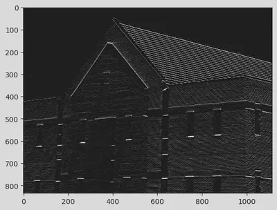
Convolve the F_x mask with the original image to obtain the x gradient of the image.
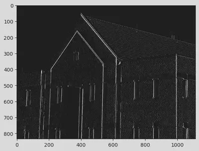
Convolve the F_y mask with the original image to obtain the y gradient of the image.
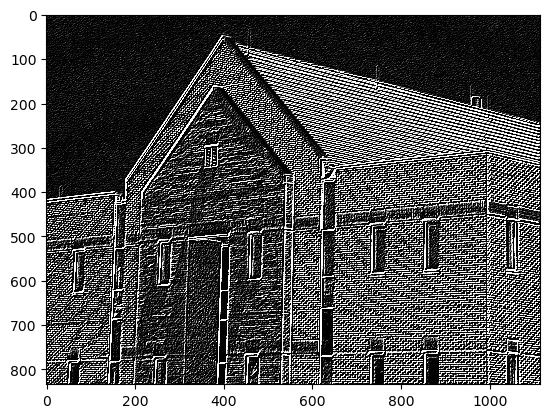
Add the results of the above two steps to obtain the combined gradient image, |g_x+g_y|.

Averaging Filter

An averaging filter is a simple low-pass filter that helps in reducing noise and blurring the image. It involves convolving the image with a suitable filter mask.

Observations

After applying the Sobel operator with the averaging filter and comparing the results obtained in step a and b, the following observations can be made:

The Sobel operator enhances the edges in the image by highlighting the changes in intensity.
The averaging filter blurs the image and reduces the noise.
When the Sobel operator is applied after the averaging filter, the edges appear smoother and less pronounced compared to applying the Sobel operator directly on the original image.
The combined gradient image, |g_x+g_y|, obtained from the Sobel operator shows the overall intensity changes in the image.

# import libraries
import numpy as np
import pandas as pd
import matplotlib.pyplot as plt
import cv2
from scipy.signal import convolve

img = cv2.imread(r"C:\Users\mpstme.student\Documents\I066\SIP\Experiment_7\Fig1016(a)(building_original).tif", 0)

cv2.imshow("Image", img)
cv2.waitKey(0)
cv2.destroyAllWindows()

Defining Horizontal and vertical masks and adding the result of the two to form a diagonal mask.

Fy = np.array([[-1, 0, 1], [-2, 0, 2], [-1, 0, 1]])

Fx = np.array([[-1, -2, -1], [0, 0, 0], [1, 2, 1]])

Fx

array([[-1, -2, -1],
       [ 0,  0,  0],
       [ 1,  2,  1]])

Fy

array([[-1,  0,  1],
       [-2,  0,  2],
       [-1,  0,  1]])

diagonal = Fx + Fy

diagonal

array([[-2, -2,  0],
       [-2,  0,  2],
       [ 0,  2,  2]])

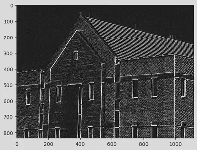
# Horizontal Edge Detection using list slicing:
img_horizontal = np.zeros([m, n])
m, n = img.shape
a = 1

for i in range(a, m - a):
  for j in range(a, n - a):
    temp = img[i - a:i + a + 1, j - a:j + a + 1]
    img_horizontal[i, j] = np.sum(np.multiply(temp, Fx))
    
plt.imshow(img_horizontal, cmap = "gray", vmin = 0, vmax = 255)

<matplotlib.image.AxesImage at 0x247ae368910>

# Horizontal Edge Detection by hardcoding the formula:
m, n = img.shape
img_horizontal = img.copy()
for i in range(1, m - 1):
  for j in range(1, n - 1):

    temp = img[i - 1, j - 1] * Fx[0, 0] + img[i - 1, j] * Fx[0, 1] + img[i - 1, j + 1] * Fx[0, 2] + \
    img[i, j - 1] * Fx[1, 0] + img[i, j] * Fx[1, 1] + img[i, j + 1] * Fx[1, 2] + \
    img[i + 1, j - 1] * Fx[2, 0] + img[i + 1, j] * Fx[2, 1] + img[i + 1, j + 1] * Fx[2, 2]
    
    temp = abs(temp)
    img_horizontal[i, j] = temp

    # Using List comprehension:
    # temp = [img[i - 1, j - 1] * mask[0, 0] + img[i - 1, j] * mask[0, 1] + img[i - 1, j + 1] * mask[0, 2] + \
    # img[i, j - 1] * mask[1, 0] + img[i, j] * mask[1, 1] + img[i, j + 1] * mask[1, 2] + \
    # img[i + 1, j - 1] * mask[2, 0] + img[i + 1, j] * mask[2, 1] + img[i + 1, j + 1] * mask[2, 2] for i in range(1, m - 1) for j in range(1, n - 1)]

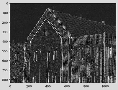
# Vertical Edge Detection using list slicing:
img_vertical = np.zeros([m, n])
m, n = img.shape
a = 1

for i in range(a, m - a):
  for j in range(a, n - a):
    temp = img[i - a:i + a + 1, j - a:j + a + 1]
    img_vertical[i, j] = np.sum(np.multiply(temp, Fy))
    
plt.imshow(img_vertical, cmap = "gray", vmin = 0, vmax = 255)

<matplotlib.image.AxesImage at 0x247ae3d6970>

# Vertical Edge Detection by hardcoding the formula:
m, n = img.shape
img_vertical = img.copy()
for i in range(1, m - 1):
  for j in range(1, n - 1):

    temp = img[i - 1, j - 1] * Fy[0, 0] + img[i - 1, j] * Fy[0, 1] + img[i - 1, j + 1] * Fy[0, 2] + \
    img[i, j - 1] * Fy[1, 0] + img[i, j] * Fy[1, 1] + img[i, j + 1] * Fy[1, 2] + \
    img[i + 1, j - 1] * Fy[2, 0] + img[i + 1, j] * Fy[2, 1] + img[i + 1, j + 1] * Fy[2, 2]
    
    temp = abs(temp)
    img_vertical[i, j] = temp

    # Using List comprehension:
    # temp = [img[i - 1, j - 1] * mask[0, 0] + img[i - 1, j] * mask[0, 1] + img[i - 1, j + 1] * mask[0, 2] + \
    # img[i, j - 1] * mask[1, 0] + img[i, j] * mask[1, 1] + img[i, j + 1] * mask[1, 2] + \
    # img[i + 1, j - 1] * mask[2, 0] + img[i + 1, j] * mask[2, 1] + img[i + 1, j + 1] * mask[2, 2] for i in range(1, m - 1) for j in range(1, n - 1)]

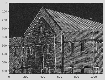
# Diagonal Edge Detection using list slicing:
img_diagonal = np.zeros([m, n])
m, n = img.shape
a = 1

for i in range(a, m - a):
  for j in range(a, n - a):
    temp = img[i - a:i + a + 1, j - a:j + a + 1]
    img_diagonal[i, j] = np.sum(np.multiply(temp, diagonal))
    
plt.imshow(img_diagonal, cmap = "gray", vmin = 0, vmax = 255)

<matplotlib.image.AxesImage at 0x247ae830af0>

# Diagonal Edge Detection by hardcoding the formula:
m, n = img.shape
img_diagonal = img.copy()
for i in range(1, m - 1):
  for j in range(1, n - 1):

    temp = img[i - 1, j - 1] * diagonal[0, 0] + img[i - 1, j] * diagonal[0, 1] + img[i - 1, j + 1] * diagonal[0, 2] + \
    img[i, j - 1] * diagonal[1, 0] + img[i, j] * diagonal[1, 1] + img[i, j + 1] * diagonal[1, 2] + \
    img[i + 1, j - 1] * diagonal[2, 0] + img[i + 1, j] * diagonal[2, 1] + img[i + 1, j + 1] * diagonal[2, 2]
    
    temp = abs(temp)
    img_diagonal[i, j] = temp

    # Using List comprehension:
    # temp = [img[i - 1, j - 1] * mask[0, 0] + img[i - 1, j] * mask[0, 1] + img[i - 1, j + 1] * mask[0, 2] + \
    # img[i, j - 1] * mask[1, 0] + img[i, j] * mask[1, 1] + img[i, j + 1] * mask[1, 2] + \
    # img[i + 1, j - 1] * mask[2, 0] + img[i + 1, j] * mask[2, 1] + img[i + 1, j + 1] * mask[2, 2] for i in range(1, m - 1) for j in range(1, n - 1)]

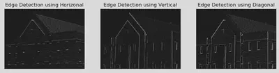
Showing the differences of Edge detection using various masks defined above (horizonal, vertical and diagonal).

radii = ["Horizonal", "Vertical", "Diagonal"]
images = [img_horizontal, img_vertical, img_diagonal]
plt.figure(figsize = (20, 10))
for i in range(len(radii)):    
    plt.subplot(1, 5, i + 1)
    plt.imshow(images[i], cmap = "gray", vmin = 0, vmax = 255)
    plt.title("Edge Detection using {}".format(radii[i]))
    plt.xticks([])
    plt.yticks([])

all_images = img_horizontal + img_vertical + img_diagonal

plt.imshow(all_images, cmap = "gray", vmin = 0, vmax = 255)

<matplotlib.image.AxesImage at 0x247ae9a41f0>

# Built in Function:
signal_x = convolve(img_horizontal, Fx, mode = "same")
signal_y = convolve(img_vertical, Fy, mode = "same")
signal_diagonal = convolve(img_diagonal, diagonal, mode = "same")
plt.imshow(signal_x, cmap = "gray", vmin = 0, vmax = 255)
plt.imshow(signal_y, cmap = "gray", vmin = 0, vmax = 255)
plt.imshow(signal_diagonal, cmap = "gray", vmin = 0, vmax = 255)

<matplotlib.image.AxesImage at 0x247bb186580>

plt.imshow(signal_y, cmap = "gray", vmin = 0, vmax = 255)

<matplotlib.image.AxesImage at 0x247bb21cfd0>

plt.imshow(signal_diagonal, cmap = "gray", vmin = 0, vmax = 255)

<matplotlib.image.AxesImage at 0x247bb254f40>

# For different sizes of masks provided from user:
size_of_mask = int(input("Enter the size of the Mask : "))
img_new = img.copy()
m, n = img.shape
print("You have requested for Mask of Size :  ", size_of_mask ,"x", size_of_mask)
a = size_of_mask//2

for i in range(a, m - a):
    for j in range(a, n - a):
        temp = np.sum(img[i - a:i + a + 1, j - a:j + a + 1])
        img_new[i, j] = temp//size_of_mask**2
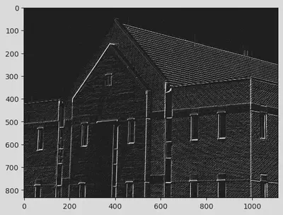
signal_x = convolve(img_new, Fx, mode = "same")
plt.imshow(signal_x, cmap = "gray", vmin = 0, vmax = 255)

Enter the size of the Mask : 5
You have requested for Mask of Size :   5 x 5

<matplotlib.image.AxesImage at 0x247b1de6a30>

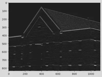
Conclusion:

As we see from the image shown above and in the cell where the difference between three types of images are shown (horizontal, vertical and diagonal, we see that the above image where we applied Averaging filter to the original image and then applied convolution seemed to detect the horizontal images better than the one in which Averaging filter wasn’t applied.

Edit this page

Image Processing Edge Detection Sobel Operator Averaging Filter