Simple Linear Regression

This README file provides instructions and information for implementing simple linear regression. The experiment involves using Python programming and various libraries.

Table of Contents

1. Aim
2. Prerequisite
3. Outcome
4. Theory
5. Task 1: Implementing Simple Linear Regression using NumPy
6. Task 2: Implementing Simple Linear Regression using Sklearn
7. Task 3: Implementing Simple Linear Regression with Dataset

Aim

The aim of this project is to implement simple linear regression.

Prerequisite

In order to complete this experiment, you should have prior knowledge of Python programming, Pandas library, Numpy library, Matplotlib, and Seaborn library.

Outcome

After successfully completing this experiment, you will be able to:

1. Implement simple linear regression using NumPy arrays.
2. Implement and verify the results using the Sklearn package.
3. Can be found here.

Theory

Linear Regression

Linear regression is a mathematical approach used to find the relationship between two or more variables. It is commonly used in machine learning to predict the behavior of a target variable based on the value of one or more predictor variables.

In simple linear regression, there is a single input variable (x) and the goal is to find a linear relationship between the input variable and the target variable (y). The relationship is represented by the equation: y = b0 + b1*x, where b0 is the intercept or bias coefficient, and b1 is the slope coefficient.

Tasks are provided to demonstrate the implementation of simple linear regression using NumPy arrays and the Sklearn package.

Task 1: Implementing Simple Linear Regression using NumPy

Perform the following tasks to implement simple linear regression using NumPy arrays:

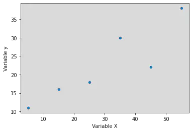
1. Define two NumPy arrays: x = [5, 15, 25, 35, 45, 55] and y = [11, 16, 18, 30, 22, 38].
2. Plot a scatter plot of x and y.
3. Compute the values of the coefficients of linear regression, b0 and b1.
4. Determine the value of r2.
5. Determine the predicted value of y for x = 20.
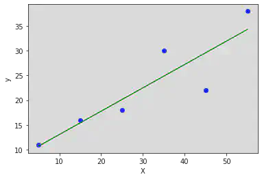
6. Plot the regression line on the scatter plot.

Task 2: Implementing Simple Linear Regression using Sklearn

Perform the following tasks to implement simple linear regression using the Sklearn package:

1. Import LinearRegression from Sklearn.
2. Reshape x to make it a two-dimensional array.
3. Create a model for linear regression.
4. Train the model using the fit() function.
5. Determine the value of r2. Compare the value with the one obtained in Task 1.
6. Determine the value of the intercept (b0) and slope (b1). Compare the values as obtained from Task 1.

Task 3: Implementing Simple Linear Regression with Dataset

Perform the following tasks to implement simple linear regression with a dataset:

1. Import sat_cgpa.csv into your notebook.
2. Explore the dataset using the head() and describe() functions.
3. Repeat steps 2 to 6 from Task 2 using the dataset.
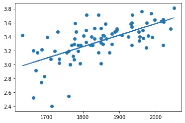
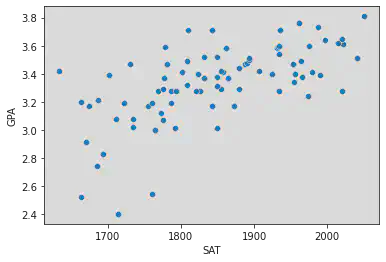
4. Import statsmodels.api.
5. Plot a scatter plot of SAT vs GPA.
6. Convert SAT into a two-dimensional array.
7. Use the OLS function from statsmodels to fit the training data to the model.
8. Print the summary of the OLS regression model.
9. Interpret the results of the OLS regression model.

Please follow the instructions above to implement simple linear regression using NumPy and Sklearn, and analyze the results using the provided dataset.

# import libraries
import matplotlib.pyplot as plt
import numpy as np
import pandas as pd
import seaborn as sns

Task 1:

x= np.array([5, 15, 25, 35, 45, 55])
y= np.array([11, 16, 18, 30, 22, 38])
sns.scatterplot(x, y)

plt.xlabel('Variable X')
plt.ylabel('Variable y')

/usr/local/lib/python3.8/dist-packages/seaborn/_decorators.py:36: FutureWarning: Pass the following variables as keyword args: x, y. From version 0.12, the only valid positional argument will be `data`, and passing other arguments without an explicit keyword will result in an error or misinterpretation.
  warnings.warn(

Text(0, 0.5, 'Variable y')

Calculation of b1 and b0 values.

x_mean = np.mean(x)
y_mean = np.mean(y)

xy = x * y

xy_mean = np.mean(xy)
x_square = x**2
x_square_mean = np.mean(x_square)

# Using Formula given in reference PDF:
b1 = ((x_mean * y_mean) - np.mean(xy))/((x_mean)**2 - x_square_mean)
print('Slope b1 is = ', b1)

b0 = y_mean - b1 * x_mean
print('Intercept b0 is = ', b0)

Slope b1 is =  nan
Intercept b0 is =  nan

<ipython-input-12-90802575e296>:11: RuntimeWarning: invalid value encountered in double_scalars
  b1 = ((x_mean * y_mean) - np.mean(xy))/((x_mean)**2 - x_square_mean)

Calculation of r square value.

# Formula:
y_pred = b1 * x + b0
error = y - y_pred
n = np.size(x)

se = (y - y_pred)**2

mse = (y - y_mean)**2

sse = np.sum(se)
ssr = np.sum(mse)

# Using Formula given in reference PDF:
r_sq = 1 - (sse/ssr)

print(se)

print(mse)

print('R square is', r_sq)

[ 0.08163265  0.32653061  4.59183673 26.44897959 57.32653061 13.79591837]
[132.25  42.25  20.25  56.25   0.25 240.25]
R square is 0.7913094027030956

plt.scatter(x, y, color = 'blue')
plt.plot(x, y_pred, color = 'green') # Plotting the Regression line
plt.xlabel('X')
plt.ylabel('y')

Text(0, 0.5, 'y')

# Formula:
x = np.array([20])
y_pred = b1 * x + b0

print(y_pred)

[nan]

Task 2:

# import libraries
from sklearn.linear_model import LinearRegression

# Converting the X array initialized in Task 1 to a 2D array.
x = x.reshape((-1, 1))

print(x)
print()
print(y)

[[ 5]
 [15]
 [25]
 [35]
 [45]
 [55]]

[11 16 18 30 22 38]

reg_model = LinearRegression()
reg_model.fit(x, y)

reg_model = LinearRegression().fit(x, y)

Hence we see that the value of R Square obtained above closely resembles to that which we obtained in Task 1.

r_sq = reg_model.score(x, y)
print("Coefficient of determination (R Square) :", r_sq)

Coefficient of determination (R Square) : 0.7913094027030955

Intercept and Slope values.

Again, these values closely resemble to those values which we obtained in Task 1 for intercept and Slope respectively.

print("Intercept (b0) :", reg_model.intercept_)
print()
print("Slope (b1) :", reg_model.coef_)

Intercept (b0) : [ 8.75 11.5 ]

Slope (b1) : [[0.1375 0.1375]
 [0.275  0.275 ]]

Task 3:

# import libraries
import statsmodels.api as sm

# Reading the File:
df = pd.read_csv("/content/sat_cgpa.csv")

# Size
df.size

168

# Shape
df.shape

(84, 2)

# Data Types
df.dtypes

SAT      int64
GPA    float64
dtype: object

df.head

<bound method NDFrame.head of      SAT   GPA
0   1714  2.40
1   1664  2.52
2   1760  2.54
3   1685  2.74
4   1693  2.83
..   ...   ...
79  1936  3.71
80  1810  3.71
81  1987  3.73
82  1962  3.76
83  2050  3.81

[84 rows x 2 columns]>

df.describe

<bound method NDFrame.describe of      SAT   GPA
0   1714  2.40
1   1664  2.52
2   1760  2.54
3   1685  2.74
4   1693  2.83
..   ...   ...
79  1936  3.71
80  1810  3.71
81  1987  3.73
82  1962  3.76
83  2050  3.81

[84 rows x 2 columns]>

sat_data = df["SAT"]
gpa_data = df["GPA"]
sns.scatterplot(sat_data, gpa_data)

/usr/local/lib/python3.8/dist-packages/seaborn/_decorators.py:36: FutureWarning: Pass the following variables as keyword args: x, y. From version 0.12, the only valid positional argument will be `data`, and passing other arguments without an explicit keyword will result in an error or misinterpretation.
  warnings.warn(

<matplotlib.axes._subplots.AxesSubplot at 0x7f2cccf39130>

x = df["SAT"]
y = df["GPA"]

x_mean = np.mean(x)
y_mean = np.mean(y)

xy = x * y

xy_mean = np.mean(xy)
x_square = x**2
x_square_mean = np.mean(x_square)

# Using Formula given in reference PDF:
b1 = ((x_mean * y_mean) - np.mean(xy))/((x_mean)**2 - x_square_mean)
print('Slope b1 is = ', b1)

b0 = y_mean - b1 * x_mean
print('Intercept b0 is = ', b0)

r_sq = 1 - (np.sum((y - y_pred) ** 2) / np.sum((y - y_mean) ** 2))
print('R Value = ', r_sq)

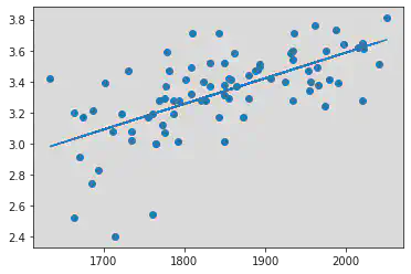
plt.scatter(x, y)
plt.plot(x, y_pred)

plt.show()

Slope b1 is =  0.0016556880500927249
Intercept b0 is =  0.27504029966044463
R Value =  0.40600391479679776

x = df["SAT"].values.reshape(-1, 1)

z = sm.add_constant(x) # Adds one more column with name 'const' to the dataset with value 1. It is an alternative addition to the reshape function which is generally used.
model = sm.OLS(df["GPA"], z) # Using the OLS Function.
# In the above line, you can store df["GPA"] in variable y to make the model syntax look readable:
# It will look like this : model = sm.OLS(y, z)
results = model.fit()

print(results.summary())

                            OLS Regression Results                            
==============================================================================
Dep. Variable:                    GPA   R-squared:                       0.406
Model:                            OLS   Adj. R-squared:                  0.399
Method:                 Least Squares   F-statistic:                     56.05
Date:                Thu, 02 Feb 2023   Prob (F-statistic):           7.20e-11
Time:                        05:24:59   Log-Likelihood:                 12.672
No. Observations:                  84   AIC:                            -21.34
Df Residuals:                      82   BIC:                            -16.48
Df Model:                           1                                         
Covariance Type:            nonrobust                                         
==============================================================================
                 coef    std err          t      P>|t|      [0.025      0.975]
------------------------------------------------------------------------------
const          0.2750      0.409      0.673      0.503      -0.538       1.088
x1             0.0017      0.000      7.487      0.000       0.001       0.002
==============================================================================
Omnibus:                       12.839   Durbin-Watson:                   0.950
Prob(Omnibus):                  0.002   Jarque-Bera (JB):               16.155
Skew:                          -0.722   Prob(JB):                     0.000310
Kurtosis:                       4.590   Cond. No.                     3.29e+04
==============================================================================

Notes:
[1] Standard Errors assume that the covariance matrix of the errors is correctly specified.
[2] The condition number is large, 3.29e+04. This might indicate that there are
strong multicollinearity or other numerical problems.

Interpretation of the result/summary generated:

The OLS regression model shows that there is a positive correlation between SAT scores and GPA.

The coefficient for SAT (0.0017) is positive, meaning that an increase in SAT score leads to an increase in GPA.

The R-squared value (0.406) indicates that 40.6% of the variance in GPA is explained by the variance in SAT scores.

We also notice that the R-squared value obtained in the OLS Regression Results summary as well as the value obtained in the cell above (for R Square) is the same. Hence, we verify that the R-squared value calculated using sklearn model and OLS Model Regresssion are the same.

Null Hypothesis is 1, Slope is not 0 as Probability = 0.000 is less than the Level of Significance (L.O.S) and hence we accept alternate hypothesis.

The greater the level of R, better the movel, i.e R should be closer to 1 than 1.