Multiple Linear Regression
Exploring Multivariate Linear Regression Modeling
 Program output
Multiple Linear Regression
This README file provides instructions and information for implementing multiple linear regression. The experiment requires knowledge of multiple linear regression concepts and aims to develop skills in implementing and interpreting the results of different models.
Table of Contents
- Aim
- Prerequisite
- Outcome
- Theory
- Task 1: Relationships between the different features
- Task 2: Fitting different simple linear regression models
- Task 3: Multiple regression model
- Task 4: Multiple regression model on 50 startups dataset
Aim
The aim of this project is to implement multiple linear regression.
Prerequisite
To successfully complete this experiment, you should have a good understanding of multiple linear regression concepts.
Outcome
After successfully completing this experiment, you will be able to:
- Implement multiple linear regression using the
sklearnpackage andstatsmodels. - Interpret the results obtained from different models and choose the best model for a given dataset.
- Can be found here.
Theory
Linear Regression
Multiple regression is an extension of simple linear regression. In multiple linear regression, a linear regression model contains more than one predictor variable. The model varies linearly with the change in the parameters β0, β1, β2, and so on. The intercept of the plane is represented by the parameter β0, while parameters β1, β2, etc. are referred to as partial regression coefficients.
The steps for multiple linear regression are as follows:
- Identify the independent and dependent variables.
- Check the relationships between the independent variables and the dependent variable using scatter plots and correlations.
- Check the relationships between the independent variables using scatter plots and correlations.
- Conduct simple linear regression for each independent variable-dependent variable pair.
- Use the non-redundant independent variables in the analysis to find the best fitting model.
- Use the best fitting model to make predictions about the dependent variable.
Tasks are provided to help you understand and implement multiple linear regression.
Task 1: Relationships between the different features
Perform the following tasks to understand the relationships between the different features:
- Import the relevant libraries.
- Load the
MLR_data.csvdataset into your notebook. - Perform exploratory data analysis (EDA) on the dataset using the
head(),shape, anddescribe()functions. - Identify the independent variables (IV) and dependent variable (DV) and plot scatter plots of IV vs. DV. Write your inferences for each plot.
- Plot scatter plots for IV vs. IV. Write your inferences for each plot.
Task 2: Fitting different simple linear regression models
Perform the following tasks to fit different simple linear regression models for each IV/DV pair:
- Import
LinearRegressionfromsklearn. - Create a model for linear regression.
- Conduct simple linear regression for each IV/DV pair:
- Interest rate vs. stock index price
- Unemployment vs. stock index price
- Determine and tabulate the values of R2, slope, and intercept for each model.
- Determine the predicted value of stock index price for an interest rate of 2.75.
- Determine the predicted value of stock index price for an unemployment rate of 6.
- Compare both models based on R2 and the mean square error between predicted and actual stock index price.
Task 3: Multiple regression model
Perform the following tasks to create a multiple regression model:
- Use both interest rate and unemployment rate as independent variables and create a multiple regression model.
- Determine the value of R2, slope, and intercept for the model.
- Determine the predicted value of stock index price for:
- Interest rate = 2.75 and unemployment rate = 5.3
- Interest rate = 2 and unemployment rate = 6
- Compare the model with the models from Task 2.
- Identify and state the best model for the dataset.
Task 4: Multiple regression model on 50 startups dataset
Perform the following tasks to create a multiple regression model on the 50 startups dataset:
- Load the 50 startups dataset.
- Follow the steps mentioned in the theory for multiple linear regression to determine the best fitting model for this dataset.
[!NOTE] Make sure to follow the instructions provided for each task and analyze the results accordingly to gain a better understanding of multiple linear regression.
# import libraries
import matplotlib.pyplot as plt
import numpy as np
import pandas as pd
import seaborn as sns
Task 1:
# Reading the File:
df = pd.read_csv("/content/MLR_data.csv")
EDA
# Size
df.size
120
# Shape
df.shape
(24, 5)
# Data Types
df.dtypes
Year int64
Month int64
Interest_Rate float64
Unemployment_Rate float64
Stock_Index_Price int64
dtype: object
df.describe()
| R&D Spend | Administration | Marketing Spend | Profit | |
|---|---|---|---|---|
| count | 50.000000 | 50.000000 | 50.000000 | 50.000000 |
| mean | 73721.615600 | 121344.639600 | 211025.097800 | 112012.639200 |
| std | 45902.256482 | 28017.802755 | 122290.310726 | 40306.180338 |
| min | 0.000000 | 51283.140000 | 0.000000 | 14681.400000 |
| 25% | 39936.370000 | 103730.875000 | 129300.132500 | 90138.902500 |
| 50% | 73051.080000 | 122699.795000 | 212716.240000 | 107978.190000 |
| 75% | 101602.800000 | 144842.180000 | 299469.085000 | 139765.977500 |
| max | 165349.200000 | 182645.560000 | 471784.100000 | 192261.830000 |
<script>
const buttonEl =
document.querySelector('#df-788e5ed7-4f2a-4876-a38d-c975b44009e3 button.colab-df-convert');
buttonEl.style.display =
google.colab.kernel.accessAllowed ? 'block' : 'none';
async function convertToInteractive(key) {
const element = document.querySelector('#df-788e5ed7-4f2a-4876-a38d-c975b44009e3');
const dataTable =
await google.colab.kernel.invokeFunction('convertToInteractive',
[key], {});
if (!dataTable) return;
const docLinkHtml = 'Like what you see? Visit the ' +
'<a target="_blank" href=https://colab.research.google.com/notebooks/data_table.ipynb>data table notebook</a>'
+ ' to learn more about interactive tables.';
element.innerHTML = '';
dataTable['output_type'] = 'display_data';
await google.colab.output.renderOutput(dataTable, element);
const docLink = document.createElement('div');
docLink.innerHTML = docLinkHtml;
element.appendChild(docLink);
}
</script>
</div>
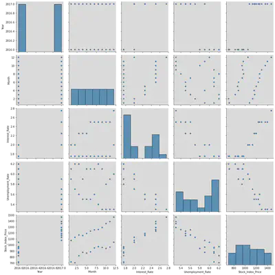
The Dependent variable is the Stock_Index_Price and the other variables are the columns other than the Stock_Index_Price.
We need to see which Independent variables best describe the Dependent variable by eliminating the redundant ones which don’t express the IV at all.
Conclusion:
We notice that from the pair plot given below, the correlation of Year and Month (Independent variables) with the Stock_Price_Index(Dependent Variable) doesn’t give us essential information to proceed and build models based on them,.
Whereas, Interest_Rate and Unemployment_Rate on the other hand, give us valuable information to proceed build models with Dependent Variables.
The graphs of Year and Month show a constant slope with no variations in them, hence they don’t describe the independent variable effectively at all.
sns.pairplot(df, height = 3, diag_kind = 'hist')
<seaborn.axisgrid.PairGrid at 0x7ff9c8049610>
Task 2:
# import libraries
from sklearn.linear_model import LinearRegression
Month_data = df["Month"]
Interest_rate_data = df["Interest_Rate"]
Unemployment_Rate_data = df["Unemployment_Rate"]
Stock_Index_Price_data = df["Stock_Index_Price"]

# Converting the X array initialized in Task 1 to a 2D arrays.
MD = Month_data.values.reshape((-1, 1))
ID = Interest_rate_data.values.reshape((-1, 1))
URD = Unemployment_Rate_data.values.reshape((-1, 1))
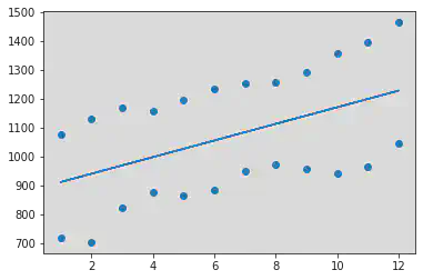
We notice a positive correlation between the two variables - Month and Stock Index Price:
reg_model = LinearRegression()
reg_model.fit(MD, Stock_Index_Price_data)

reg_model = LinearRegression().fit(MD, Stock_Index_Price_data)
r_sq = reg_model.score(MD, Stock_Index_Price_data)
print("R Square Value : ", r_sq)
b0 = reg_model.intercept_
b1 = reg_model.coef_
print("Intercept (b0) :", reg_model.intercept_)
print()
print("Slope (b1) :", reg_model.coef_)
R Square Value : 0.23163745862450869
Intercept (b0) : 883.1287878787878
Slope (b1) : [28.76223776]
y_pred = b1 * MD + b0
plt.scatter(MD, Stock_Index_Price_data)
plt.plot(MD, y_pred)

plt.show()
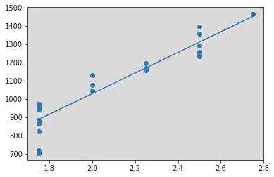
We notice a positive correlation between the two variables - Interest Rate and Stock Index Price:
reg_model = LinearRegression()
reg_model.fit(ID, Stock_Index_Price_data)

reg_model = LinearRegression().fit(ID, Stock_Index_Price_data)

r_sq = reg_model.score(ID, Stock_Index_Price_data)
print("R Square Value : ", r_sq)
print("Intercept (b0) :", reg_model.intercept_)
print()
print("Slope (b1) :", reg_model.coef_)
R Square Value : 0.8757089547891359
Intercept (b0) : -99.46431881371655
Slope (b1) : [564.20389249]
b0 = reg_model.intercept_
b1 = reg_model.coef_
y_pred = b1 * ID + b0
plt.scatter(ID, Stock_Index_Price_data)
plt.plot(ID, y_pred)

plt.show()
ID = 2.75
y_pred = b1 * ID + b0
MSE = ((y_pred - 1464 )**2)/2
print(MSE)
[70.84801858]
We notice a negative correlation between the two variables - Unemployment Rate and Stock Index Price:
reg_model = LinearRegression()
reg_model.fit(URD, Stock_Index_Price_data)

reg_model = LinearRegression().fit(URD, Stock_Index_Price_data)

r_sq = reg_model.score(URD, Stock_Index_Price_data)
print("R Square Value : ", r_sq)
print("Intercept (b0) :", reg_model.intercept_)
print()
print("Slope (b1) :", reg_model.coef_)
R Square Value : 0.850706607677214
Intercept (b0) : 4471.339321357287
Slope (b1) : [-588.96207585]
b0 = reg_model.intercept_
b1 = reg_model.coef_
y_pred = b1 * URD + b0
plt.scatter(URD, Stock_Index_Price_data)
plt.plot(URD, y_pred)

plt.show()
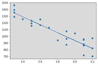
URD = 6
y_pred = b1 * URD + b0
MSE = ((y_pred - 1047 )**2)/2
print(MSE)
[5987.80537926]
Task 3:
Multiple Regression Model of Interest Rate and Unemployment Rate with Stock Index Price:
x = np.array(df[["Interest_Rate", "Unemployment_Rate"]])
y = np.array(df["Stock_Index_Price"])
reg_model.fit(x, y)
r_sq = reg_model.score(x, y)
print("R Square Value : ", r_sq)
b0 = reg_model.intercept_
b1 = reg_model.coef_[0]
b2 = reg_model.coef_[1]

print("Intercept (b0) :", reg_model.intercept_)
print()
print(b1)
print(b2)

r_sq = reg_model.score(x, y)
print("R Square Value : ", r_sq)
b0 = reg_model.intercept_
b1 = reg_model.coef_[0]
b2 = reg_model.coef_[1]

print("Intercept (b0) :", reg_model.intercept_)
print()
print(b1)
print(b2)
y_pred = b0 + b1*2.75 + b2 * 5.3
print(y_pred)
y_pred = b0 + b1*2 + b2 * 6
print(y_pred)
R Square Value : 0.8976335894170216
Intercept (b0) : 1798.4039776258544
345.54008701056574
-250.14657136938055
R Square Value : 0.8976335894170216
Intercept (b0) : 1798.4039776258544
345.54008701056574
-250.14657136938055
1422.8623886471935
988.6047234307027
Multiple Regression Model of Interest Rate, Unemployment Rate and Month with Stock Index Price:
x = np.array(df[["Interest_Rate", "Unemployment_Rate", "Month"]])
y = np.array(df["Stock_Index_Price"])
reg_model.fit(x, y)

r_sq = reg_model.score(x, y)
print("R Square Value : ", r_sq)
b0 = reg_model.intercept_
b1 = reg_model.coef_[0]
b2 = reg_model.coef_[1]
b3 = reg_model.coef_[2]

print("Intercept (b0) :", reg_model.intercept_)
print()
print(b1)
print(b2)
print(b3)
y_pred = b0 + b1*2.75 + b2 * 5.3 + b3 * 12
print(y_pred)
y_pred = b0 + b1*2 + b2 * 6 + b3 * 12
print(y_pred)
R Square Value : 0.9230425469229033
Intercept (b0) : 1591.5963382763719
335.1930601634653
-222.08250237506545
10.182486970633022
1458.529834785651
1051.677288000506
Hence we can conclude from the above 2 models that the model which includes month as a independent variable is more suitable as it’s R value = 0.923 which is greater than the R value of the model without month as a independent variable (0.897).
Task 4:
# Reading the File:
df = pd.read_csv("/content/50_Startups.csv")
df1 = pd.read_csv("/content/50_Startups.csv")
EDA
# Size
df.size
250
# Shape
df.shape
(50, 5)
# Data Types
df.dtypes
R&D Spend float64
Administration float64
Marketing Spend float64
State object
Profit float64
dtype: object
df.describe()
| R&D Spend | Administration | Marketing Spend | Profit | |
|---|---|---|---|---|
| count | 50.000000 | 50.000000 | 50.000000 | 50.000000 |
| mean | 73721.615600 | 121344.639600 | 211025.097800 | 112012.639200 |
| std | 45902.256482 | 28017.802755 | 122290.310726 | 40306.180338 |
| min | 0.000000 | 51283.140000 | 0.000000 | 14681.400000 |
| 25% | 39936.370000 | 103730.875000 | 129300.132500 | 90138.902500 |
| 50% | 73051.080000 | 122699.795000 | 212716.240000 | 107978.190000 |
| 75% | 101602.800000 | 144842.180000 | 299469.085000 | 139765.977500 |
| max | 165349.200000 | 182645.560000 | 471784.100000 | 192261.830000 |
<script>
const buttonEl =
document.querySelector('#df-f7641fe5-e1da-4911-9a09-a0935daf9629 button.colab-df-convert');
buttonEl.style.display =
google.colab.kernel.accessAllowed ? 'block' : 'none';
async function convertToInteractive(key) {
const element = document.querySelector('#df-f7641fe5-e1da-4911-9a09-a0935daf9629');
const dataTable =
await google.colab.kernel.invokeFunction('convertToInteractive',
[key], {});
if (!dataTable) return;
const docLinkHtml = 'Like what you see? Visit the ' +
'<a target="_blank" href=https://colab.research.google.com/notebooks/data_table.ipynb>data table notebook</a>'
+ ' to learn more about interactive tables.';
element.innerHTML = '';
dataTable['output_type'] = 'display_data';
await google.colab.output.renderOutput(dataTable, element);
const docLink = document.createElement('div');
docLink.innerHTML = docLinkHtml;
element.appendChild(docLink);
}
</script>
</div>
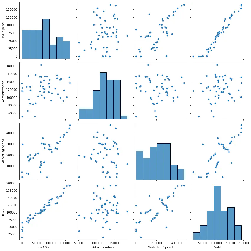
The Dependent variable is the Profit and the other variables are the columns other than the Stock_Index_Price.
We need to see which Independent variables best describe the Dependent variable by eliminating the redundant ones which don’t express the IV at all.
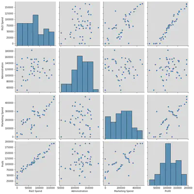
Conclusion:
We notice that from the pair plot given below, the correlation of Administration and State (Independent variables) with the Profit(Dependent Variable) doesn’t give us essential information to proceed and build models based on them.
Whereas, R&D Spend and Marketing Spend on the other hand, give us valuable information to proceed build models with Dependent Variables.
The graphs of Administration and State show a constant slope with no variations in them, hence they don’t describe the independent variable effectively at all.
sns.pairplot(df, height = 3, diag_kind = 'hist')
<seaborn.axisgrid.PairGrid at 0x7ff98945ae20>
x = np.array(df[['R&D Spend', 'Administration', 'Marketing Spend']])
y = np.array(df['Profit'])
reg_model = LinearRegression()

reg_model.fit(x, y)

r_sq = reg_model.score(x, y)
print("R Square Value : ", r_sq)
b0 = reg_model.intercept_
b1 = reg_model.coef_[0]
b2 = reg_model.coef_[1]
b3 = reg_model.coef_[2]

print("Intercept (b0) :", reg_model.intercept_)
print()
print(b1)
print(b2)
print(b3)
y_pred = b0 + b1*2.75 + b2 * 5.3 + b3 * 12
print(y_pred)
y_pred = b0 + b1*2 + b2 * 6 + b3 * 12
print(y_pred)
R Square Value : 0.9507459940683246
Intercept (b0) : 50122.19298986524
0.8057150499157437
-0.02681596839475075
0.027228064800818817
50124.59331839763
50123.970260932314
Hence we can conclude that the Multiple Regression model with the respective columns are helpful in building a good model (with r value 0.95).
import statsmodels.api as sm
results = sm.OLS(y, x).fit()
print(results.summary())
OLS Regression Results
=======================================================================================
Dep. Variable: y R-squared (uncentered): 0.987
Model: OLS Adj. R-squared (uncentered): 0.987
Method: Least Squares F-statistic: 1232.
Date: Thu, 09 Feb 2023 Prob (F-statistic): 1.17e-44
Time: 12:35:27 Log-Likelihood: -545.82
No. Observations: 50 AIC: 1098.
Df Residuals: 47 BIC: 1103.
Df Model: 3
Covariance Type: nonrobust
==============================================================================
coef std err t P>|t| [0.025 0.975]
------------------------------------------------------------------------------
x1 0.7180 0.065 11.047 0.000 0.587 0.849
x2 0.3277 0.031 10.458 0.000 0.265 0.391
x3 0.0822 0.022 3.733 0.001 0.038 0.126
==============================================================================
Omnibus: 0.665 Durbin-Watson: 1.361
Prob(Omnibus): 0.717 Jarque-Bera (JB): 0.749
Skew: -0.126 Prob(JB): 0.688
Kurtosis: 2.456 Cond. No. 9.76
==============================================================================
Notes:
[1] R² is computed without centering (uncentered) since the model does not contain a constant.
[2] Standard Errors assume that the covariance matrix of the errors is correctly specified.
Conclusion
From the above experiment, I learnt the following:
- Implement multiple linear regression by using sklearn package statsmodels.
- Interpret the results obtained from different models and choose the best model for the given data set using R values and P with reference to L.O.S.
Srihari Thyagarajan
B Tech AI Senior Student
Hi, I’m Haleshot, a senior-year student studying B Tech Artificial Intelligence. I like projects relating to ML, AI, DL, CV, NLP, Image Processing, etc. Currently exploring Python, FastAPI, projects involving AI and platforms such as HuggingFace and Kaggle.