Naive Bayes Classification
Exploring the Naïve Bayes Algorithm for Classification Tasks
 Program output
Naïve Bayes Algorithm for Classification
This README file provides instructions and information for implementing the Naïve Bayes algorithm for classification. The experiment requires prior knowledge of Python programming and the following libraries: Pandas, NumPy, Matplotlib, and Seaborn.
Table of Contents
Aim
The aim of this project is to implement the Naïve Bayes algorithm for classification.
Prerequisite
To successfully complete this experiment, you should have knowledge of Python programming and the following libraries: Pandas, NumPy, Matplotlib, and Seaborn.
Outcome
After successfully completing this experiment, you will be able to:
- Implement the Naïve Bayes technique for classification.
- Compare the results of Naïve Bayes and KNN algorithms.
- Understand and infer the results of different classification metrics.
- Can be found here.
Theory
Naïve Bayes Classifier
The Naïve Bayes algorithm is a supervised learning algorithm based on Bayes’ theorem. It is used for solving classification problems and is particularly effective for text classification with high-dimensional training datasets. The Naïve Bayes Classifier is a simple yet effective classification algorithm that can build fast machine learning models for quick predictions. It is a probabilistic classifier that predicts based on the probability of an object. Examples of Naïve Bayes applications include spam filtration, sentiment analysis, and article classification.
Bayes’ Theorem
Bayes’ theorem, also known as Bayes’ Rule or Bayes’ law, is used to determine the probability of a hypothesis given prior knowledge. It relies on conditional probability. The formula for Bayes’ theorem is as follows:
P(A|B) = (P(B|A) * P(A)) / P(B)
Where:
- P(A|B) is the posterior probability: the probability of hypothesis A given the observed event B.
- P(B|A) is the likelihood probability: the probability of the evidence given that the probability of a hypothesis A is true.
- P(A) is the prior probability: the probability of the hypothesis before observing the evidence.
- P(B) is the marginal probability: the probability of the evidence.
Working of Naïve Bayes Classifier
The working of the Naïve Bayes Classifier involves the following steps:
- Convert the given dataset into frequency tables.
- Generate a likelihood table by finding the probabilities of given features.
- Use Bayes’ theorem to calculate the posterior probability.
Tasks
Perform the following tasks to implement the Naïve Bayes algorithm and compare it with KNN:
Task 1: Implementing Naïve Bayes Algorithm on Car Dataset
- Apply the Naïve Bayes algorithm to the given car dataset.
- Show all the steps of the training phase.
- Identify the class for the test data point (color = Yellow, Type = Sports, Origin = Domestic).
- Solve the answer on paper and upload the image.
Task 2: Operations on Adult.csv Dataset
- Upload the dataset into a dataframe.
- Check the shape of the dataset.
- Find out all the categorical columns from the dataset.
- Check if null values exist in all the categorical columns.
- Identify the problems with the “workclass,” “Occupation,” and “native_country” columns and rectify them.
- Explore numeric columns and check for any null values.
- Create a feature vector with x = all the columns except income and y = income.
- Implement feature engineering for the train-test split dataset:
- Check the data types of columns of the input features of the training dataset.
- Identify categorical columns that have null values and fill them with the most probable value in the dataset.
- Repeat the above step for the input features of the test dataset.
- Apply one-hot encoding on all the categorical columns.
- Apply feature scaling using a robust scaler.
Task 3: Implement KNN Algorithm on Sklearn Dataset with k=5.
Task 4: Implement Naïve Bayes Algorithm on the given dataset.
Task 5: Compare the confusion matrix for both classifiers.
Task 6: Compare the accuracy score of both classifiers.
Task 7: Draw the ROC curve to compare both models.
Follow the instructions provided for each task and analyze the results to gain a better understanding of the Naïve Bayes algorithm and its comparison with KNN.
# import libraries
import matplotlib.pyplot as plt
import numpy as np
import pandas as pd
import seaborn as sns
# Reading the Dataset and loading as a dataframe.
df = pd.read_csv("/content/adultPrac7.csv")
EDA:
df.shape
(32561, 15)
df.head(15)
| age | workclass | fnlwgt | education | education_num | marital_status | occupation | relationship | race | sex | capital_gain | capital_loss | hours_per_week | native_country | income | |
|---|---|---|---|---|---|---|---|---|---|---|---|---|---|---|---|
| 0 | 39 | State-gov | 77516 | Bachelors | 13 | Never-married | Adm-clerical | Not-in-family | White | Male | 2174 | 0 | 40 | United-States | <=50K |
| 1 | 50 | Self-emp-not-inc | 83311 | Bachelors | 13 | Married-civ-spouse | Exec-managerial | Husband | White | Male | 0 | 0 | 13 | United-States | <=50K |
| 2 | 38 | Private | 215646 | HS-grad | 9 | Divorced | Handlers-cleaners | Not-in-family | White | Male | 0 | 0 | 40 | United-States | <=50K |
| 3 | 53 | Private | 234721 | 11th | 7 | Married-civ-spouse | Handlers-cleaners | Husband | Black | Male | 0 | 0 | 40 | United-States | <=50K |
| 4 | 28 | Private | 338409 | Bachelors | 13 | Married-civ-spouse | Prof-specialty | Wife | Black | Female | 0 | 0 | 40 | Cuba | <=50K |
| 5 | 37 | Private | 284582 | Masters | 14 | Married-civ-spouse | Exec-managerial | Wife | White | Female | 0 | 0 | 40 | United-States | <=50K |
| 6 | 49 | Private | 160187 | 9th | 5 | Married-spouse-absent | Other-service | Not-in-family | Black | Female | 0 | 0 | 16 | Jamaica | <=50K |
| 7 | 52 | Self-emp-not-inc | 209642 | HS-grad | 9 | Married-civ-spouse | Exec-managerial | Husband | White | Male | 0 | 0 | 45 | United-States | >50K |
| 8 | 31 | Private | 45781 | Masters | 14 | Never-married | Prof-specialty | Not-in-family | White | Female | 14084 | 0 | 50 | United-States | >50K |
| 9 | 42 | Private | 159449 | Bachelors | 13 | Married-civ-spouse | Exec-managerial | Husband | White | Male | 5178 | 0 | 40 | United-States | >50K |
| 10 | 37 | Private | 280464 | Some-college | 10 | Married-civ-spouse | Exec-managerial | Husband | Black | Male | 0 | 0 | 80 | United-States | >50K |
| 11 | 30 | State-gov | 141297 | Bachelors | 13 | Married-civ-spouse | Prof-specialty | Husband | Asian-Pac-Islander | Male | 0 | 0 | 40 | India | >50K |
| 12 | 23 | Private | 122272 | Bachelors | 13 | Never-married | Adm-clerical | Own-child | White | Female | 0 | 0 | 30 | United-States | <=50K |
| 13 | 32 | Private | 205019 | Assoc-acdm | 12 | Never-married | Sales | Not-in-family | Black | Male | 0 | 0 | 50 | United-States | <=50K |
| 14 | 40 | Private | 121772 | Assoc-voc | 11 | Married-civ-spouse | Craft-repair | Husband | Asian-Pac-Islander | Male | 0 | 0 | 40 | ? | >50K |
<script>
const buttonEl =
document.querySelector('#df-fcb0abcf-ffa6-485a-99ef-105a201cac75 button.colab-df-convert');
buttonEl.style.display =
google.colab.kernel.accessAllowed ? 'block' : 'none';
async function convertToInteractive(key) {
const element = document.querySelector('#df-fcb0abcf-ffa6-485a-99ef-105a201cac75');
const dataTable =
await google.colab.kernel.invokeFunction('convertToInteractive',
[key], {});
if (!dataTable) return;
const docLinkHtml = 'Like what you see? Visit the ' +
'<a target="_blank" href=https://colab.research.google.com/notebooks/data_table.ipynb>data table notebook</a>'
+ ' to learn more about interactive tables.';
element.innerHTML = '';
dataTable['output_type'] = 'display_data';
await google.colab.output.renderOutput(dataTable, element);
const docLink = document.createElement('div');
docLink.innerHTML = docLinkHtml;
element.appendChild(docLink);
}
</script>
</div>
df.dtypes
age int64
workclass object
fnlwgt int64
education object
education_num int64
marital_status object
occupation object
relationship object
race object
sex object
capital_gain int64
capital_loss int64
hours_per_week int64
native_country object
income object
dtype: object
df.describe
<bound method NDFrame.describe of age workclass fnlwgt education education_num \
0 39 State-gov 77516 Bachelors 13
1 50 Self-emp-not-inc 83311 Bachelors 13
2 38 Private 215646 HS-grad 9
3 53 Private 234721 11th 7
4 28 Private 338409 Bachelors 13
... ... ... ... ... ...
32556 27 Private 257302 Assoc-acdm 12
32557 40 Private 154374 HS-grad 9
32558 58 Private 151910 HS-grad 9
32559 22 Private 201490 HS-grad 9
32560 52 Self-emp-inc 287927 HS-grad 9
marital_status occupation relationship race \
0 Never-married Adm-clerical Not-in-family White
1 Married-civ-spouse Exec-managerial Husband White
2 Divorced Handlers-cleaners Not-in-family White
3 Married-civ-spouse Handlers-cleaners Husband Black
4 Married-civ-spouse Prof-specialty Wife Black
... ... ... ... ...
32556 Married-civ-spouse Tech-support Wife White
32557 Married-civ-spouse Machine-op-inspct Husband White
32558 Widowed Adm-clerical Unmarried White
32559 Never-married Adm-clerical Own-child White
32560 Married-civ-spouse Exec-managerial Wife White
sex capital_gain capital_loss hours_per_week native_country \
0 Male 2174 0 40 United-States
1 Male 0 0 13 United-States
2 Male 0 0 40 United-States
3 Male 0 0 40 United-States
4 Female 0 0 40 Cuba
... ... ... ... ... ...
32556 Female 0 0 38 United-States
32557 Male 0 0 40 United-States
32558 Female 0 0 40 United-States
32559 Male 0 0 20 United-States
32560 Female 15024 0 40 United-States
income
0 <=50K
1 <=50K
2 <=50K
3 <=50K
4 <=50K
... ...
32556 <=50K
32557 >50K
32558 <=50K
32559 <=50K
32560 >50K
[32561 rows x 15 columns]>
df.info()
<class 'pandas.core.frame.DataFrame'>
RangeIndex: 32561 entries, 0 to 32560
Data columns (total 15 columns):
# Column Non-Null Count Dtype
--- ------ -------------- -----
0 age 32561 non-null int64
1 workclass 32561 non-null object
2 fnlwgt 32561 non-null int64
3 education 32561 non-null object
4 education_num 32561 non-null int64
5 marital_status 32561 non-null object
6 occupation 32561 non-null object
7 relationship 32561 non-null object
8 race 32561 non-null object
9 sex 32561 non-null object
10 capital_gain 32561 non-null int64
11 capital_loss 32561 non-null int64
12 hours_per_week 32561 non-null int64
13 native_country 32561 non-null object
14 income 32561 non-null object
dtypes: int64(6), object(9)
memory usage: 3.7+ MB
# Checking Labels in workclass variable:
df.workclass.unique()
array([' State-gov', ' Self-emp-not-inc', ' Private', ' Federal-gov',
' Local-gov', ' ?', ' Self-emp-inc', ' Without-pay',
' Never-worked'], dtype=object)
# Showing the Value counts of each category of each workclass category.
df.workclass.value_counts()
Private 22696
Self-emp-not-inc 2541
Local-gov 2093
? 1836
State-gov 1298
Self-emp-inc 1116
Federal-gov 960
Without-pay 14
Never-worked 7
Name: workclass, dtype: int64
# To replace the '?' with NaN values as that can be handled by pandas library.
df['workclass'].replace(' ?', np.NaN, inplace = True)
df.workclass.value_counts()
Private 22696
Self-emp-not-inc 2541
Local-gov 2093
State-gov 1298
Self-emp-inc 1116
Federal-gov 960
Without-pay 14
Never-worked 7
Name: workclass, dtype: int64
df.workclass.unique()
array([' State-gov', ' Self-emp-not-inc', ' Private', ' Federal-gov',
' Local-gov', nan, ' Self-emp-inc', ' Without-pay',
' Never-worked'], dtype=object)
df.capital_gainreplace(' ?', np.NaN, inplace = True)
# Checking for '?' value in other features
df[df == "?"].count()
age 0
workclass 0
fnlwgt 0
education 0
education_num 0
marital_status 0
occupation 0
relationship 0
race 0
sex 0
capital_gain 0
capital_loss 0
hours_per_week 0
native_country 0
income 0
dtype: int64
# X signify the features, Y signify labels
X = df.drop(['income'], axis = 1)
Y = df["income"]
X.dtypes
age int64
workclass object
fnlwgt int64
education object
education_num int64
marital_status object
occupation object
relationship object
race object
sex object
capital_gain int64
capital_loss int64
hours_per_week int64
native_country object
dtype: object
Y.dtypes
dtype('O')
# Displaying the categorical features:
categorical = [col for col in X.columns if X[col].dtypes == 'O']
categorical
['workclass',
'education',
'marital_status',
'occupation',
'relationship',
'race',
'sex',
'native_country']
# Displaying the numerical features:
numerical = [col for col in X.columns if X[col].dtypes != 'O']
numerical
['age',
'fnlwgt',
'education_num',
'capital_gain',
'capital_loss',
'hours_per_week']
# Print percentage of missing values in the Categorical variables in the training set
X[categorical].isnull().mean()
workclass 0.056386
education 0.000000
marital_status 0.000000
occupation 0.056601
relationship 0.000000
race 0.000000
sex 0.000000
native_country 0.017905
dtype: float64
# Since these are categorical values, we cannot use mean and hence use mode to replace the Nan values:
# Three features - workclass, occupation and native_country have null values and hence we replace them with the highest freuqncy of that respective feature.
# impute the missing categorical variables with most freuqnt value:
for df2 in [X]:
  df2['workclass'].fillna(X['workclass'].mode()[0], inplace = True)
  df2['occupation'].fillna(X['occupation'].mode()[0], inplace = True)
  df2['native_country'].fillna(X['native_country'].mode()[0], inplace = True)
# Checking missing values in the feature set:
X.isnull().sum()
age 0
workclass 0
fnlwgt 0
education 0
education_num 0
marital_status 0
occupation 0
relationship 0
race 0
sex 0
capital_gain 0
capital_loss 0
hours_per_week 0
native_country 0
dtype: int64
# Now we do label encoding after eliminating all null values from the dataset:
X[categorical].head()
| workclass | education | marital_status | occupation | relationship | race | sex | native_country | |
|---|---|---|---|---|---|---|---|---|
| 0 | State-gov | Bachelors | Never-married | Adm-clerical | Not-in-family | White | Male | United-States |
| 1 | Self-emp-not-inc | Bachelors | Married-civ-spouse | Exec-managerial | Husband | White | Male | United-States |
| 2 | Private | HS-grad | Divorced | Handlers-cleaners | Not-in-family | White | Male | United-States |
| 3 | Private | 11th | Married-civ-spouse | Handlers-cleaners | Husband | Black | Male | United-States |
| 4 | Private | Bachelors | Married-civ-spouse | Prof-specialty | Wife | Black | Female | Cuba |
<script>
const buttonEl =
document.querySelector('#df-f49295aa-8869-4cdd-8ab9-f3fefae63cc9 button.colab-df-convert');
buttonEl.style.display =
google.colab.kernel.accessAllowed ? 'block' : 'none';
async function convertToInteractive(key) {
const element = document.querySelector('#df-f49295aa-8869-4cdd-8ab9-f3fefae63cc9');
const dataTable =
await google.colab.kernel.invokeFunction('convertToInteractive',
[key], {});
if (!dataTable) return;
const docLinkHtml = 'Like what you see? Visit the ' +
'<a target="_blank" href=https://colab.research.google.com/notebooks/data_table.ipynb>data table notebook</a>'
+ ' to learn more about interactive tables.';
element.innerHTML = '';
dataTable['output_type'] = 'display_data';
await google.colab.output.renderOutput(dataTable, element);
const docLink = document.createElement('div');
docLink.innerHTML = docLinkHtml;
element.appendChild(docLink);
}
</script>
</div>
from sklearn import preprocessing
label_encoder = preprocessing.LabelEncoder()

for i in X[categorical]:
  X[i] = label_encoder.fit_transform(X[i])

# The above for loop eliminates the need for transforming each categorical feature individually like this:
# X['workclass'] = label_encoder.fit_transform(X['workclass'])
# X['education'] = label_encoder.fit_transform(X['workclass'])
# X['marital_status'] = label_encoder.fit_transform(X['workclass'])
# X['occupation'] = label_encoder.fit_transform(X['workclass'])
# X['relationship'] = label_encoder.fit_transform(X['workclass'])
# X['race'] = label_encoder.fit_transform(X['workclass'])
# X['sex'] = label_encoder.fit_transform(X['workclass'])
# X['native_country'] = label_encoder.fit_transform(X['workclass'])
X.head(15)
| age | workclass | fnlwgt | education | education_num | marital_status | occupation | relationship | race | sex | capital_gain | capital_loss | hours_per_week | native_country | |
|---|---|---|---|---|---|---|---|---|---|---|---|---|---|---|
| 0 | 39 | 6 | 77516 | 9 | 13 | 4 | 0 | 1 | 4 | 1 | 2174 | 0 | 40 | 38 |
| 1 | 50 | 5 | 83311 | 9 | 13 | 2 | 3 | 0 | 4 | 1 | 0 | 0 | 13 | 38 |
| 2 | 38 | 3 | 215646 | 11 | 9 | 0 | 5 | 1 | 4 | 1 | 0 | 0 | 40 | 38 |
| 3 | 53 | 3 | 234721 | 1 | 7 | 2 | 5 | 0 | 2 | 1 | 0 | 0 | 40 | 38 |
| 4 | 28 | 3 | 338409 | 9 | 13 | 2 | 9 | 5 | 2 | 0 | 0 | 0 | 40 | 4 |
| 5 | 37 | 3 | 284582 | 12 | 14 | 2 | 3 | 5 | 4 | 0 | 0 | 0 | 40 | 38 |
| 6 | 49 | 3 | 160187 | 6 | 5 | 3 | 7 | 1 | 2 | 0 | 0 | 0 | 16 | 22 |
| 7 | 52 | 5 | 209642 | 11 | 9 | 2 | 3 | 0 | 4 | 1 | 0 | 0 | 45 | 38 |
| 8 | 31 | 3 | 45781 | 12 | 14 | 4 | 9 | 1 | 4 | 0 | 14084 | 0 | 50 | 38 |
| 9 | 42 | 3 | 159449 | 9 | 13 | 2 | 3 | 0 | 4 | 1 | 5178 | 0 | 40 | 38 |
| 10 | 37 | 3 | 280464 | 15 | 10 | 2 | 3 | 0 | 2 | 1 | 0 | 0 | 80 | 38 |
| 11 | 30 | 6 | 141297 | 9 | 13 | 2 | 9 | 0 | 1 | 1 | 0 | 0 | 40 | 18 |
| 12 | 23 | 3 | 122272 | 9 | 13 | 4 | 0 | 3 | 4 | 0 | 0 | 0 | 30 | 38 |
| 13 | 32 | 3 | 205019 | 7 | 12 | 4 | 11 | 1 | 2 | 1 | 0 | 0 | 50 | 38 |
| 14 | 40 | 3 | 121772 | 8 | 11 | 2 | 2 | 0 | 1 | 1 | 0 | 0 | 40 | 38 |
<script>
const buttonEl =
document.querySelector('#df-c3973471-34c6-4f17-a92d-092f081e2b47 button.colab-df-convert');
buttonEl.style.display =
google.colab.kernel.accessAllowed ? 'block' : 'none';
async function convertToInteractive(key) {
const element = document.querySelector('#df-c3973471-34c6-4f17-a92d-092f081e2b47');
const dataTable =
await google.colab.kernel.invokeFunction('convertToInteractive',
[key], {});
if (!dataTable) return;
const docLinkHtml = 'Like what you see? Visit the ' +
'<a target="_blank" href=https://colab.research.google.com/notebooks/data_table.ipynb>data table notebook</a>'
+ ' to learn more about interactive tables.';
element.innerHTML = '';
dataTable['output_type'] = 'display_data';
await google.colab.output.renderOutput(dataTable, element);
const docLink = document.createElement('div');
docLink.innerHTML = docLinkHtml;
element.appendChild(docLink);
}
</script>
</div>
# Now we need to normalize the data, as each feature has a varying range:
from sklearn.model_selection import train_test_split
X_train, X_test, y_train, y_test = train_test_split(X, Y, test_size = 0.3, random_state = 0)
# Checking the shape of training and testing samples after splitting
X_train.shape, X_test.shape
((22792, 14), (9769, 14))
from sklearn.preprocessing import StandardScaler
scaler = StandardScaler()
X_train = scaler.fit_transform(X_train)
X_test = scaler.fit_transform(X_test)
# Train a Gaussian Naive Bayes Classifier on the training set
from sklearn.naive_bayes import GaussianNB

# instantiate the model
gnb = GaussianNB()

# Fit the model:
gnb.fit(X_train, y_train)
GaussianNB()In a Jupyter environment, please rerun this cell to show the HTML representation or trust the notebook.
On GitHub, the HTML representation is unable to render, please try loading this page with nbviewer.org.
GaussianNB()
y_pred = gnb.predict(X_test)
y_pred
array([' <=50K', ' <=50K', ' <=50K', ..., ' >50K', ' <=50K', ' <=50K'],
dtype='<U6')
from sklearn.metrics import confusion_matrix, accuracy_score
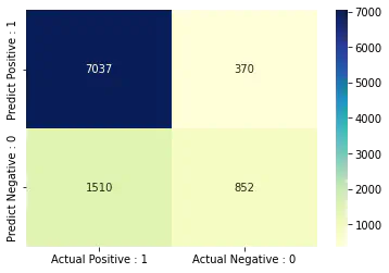
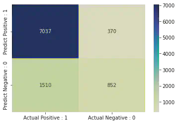
cm = confusion_matrix(y_test, y_pred)
ac = accuracy_score(y_test, y_pred)
print(cm, "\n", ac)
[[7037 370]
[1510 852]]
0.8075545091616337
print("True Positives : ", cm[0, 0])
print("True Negatives : ", cm[1, 1])
print("False Positives : ", cm[0, 1])
print("False Negatives : ", cm[1, 0])
True Positives : 7037
True Negatives : 852
False Positives : 370
False Negatives : 1510
cm_matrix = pd.DataFrame(data = cm, columns = ["Actual Positive : 1", "Actual Negative : 0"], index = ["Predict Positive : 1", "Predict Negative : 0"])
import seaborn as sns
sns.heatmap(cm_matrix, annot = True, fmt = 'd', cmap = 'YlGnBu')
<AxesSubplot:>
from sklearn.metrics import classification_report
print(classification_report(y_test, y_pred))
precision recall f1-score support
<=50K 0.82 0.95 0.88 7407
>50K 0.70 0.36 0.48 2362
accuracy 0.81 9769
macro avg 0.76 0.66 0.68 9769
weighted avg 0.79 0.81 0.78 9769
from sklearn.neighbors import KNeighborsClassifier
classifier = KNeighborsClassifier(n_neighbors = 5, p = 2) # We mention in the parameters for it to take
# 5 nearest neigbors(default value) and p = 2(default value = Eucledian distance)
classifier.fit(X_train, y_train) # Feed the training data to the classifier.
KNeighborsClassifier()In a Jupyter environment, please rerun this cell to show the HTML representation or trust the notebook.
On GitHub, the HTML representation is unable to render, please try loading this page with nbviewer.org.
KNeighborsClassifier()
y_pred = classifier.predict(X_test) # Predicting for x_test data
y_pred
array([' <=50K', ' <=50K', ' <=50K', ..., ' >50K', ' >50K', ' <=50K'],
dtype=object)
cm = confusion_matrix(y_test, y_pred)
ac = accuracy_score(y_test, y_pred)
print(cm, "\n", ac)
[[6685 722]
[ 990 1372]]
0.8247517657897431
Conclusion:
- The accuracy of Naive-Bayes is 80.7%
- The accuracy of KNN Neighbours (with k = 5) is 82.4% From the acquired results, we can conclude that KNN is better for the sample which we took in this case.
Learnt the following from the above experiment:
- Implement Naïve Bayes technique for the classification
- Compare results of Naïve Bayes and KNN
- Understand and infer results of different classification metrics
Srihari Thyagarajan
B Tech AI Senior Student
Hi, I’m Haleshot, a senior-year student studying B Tech Artificial Intelligence. I like projects relating to ML, AI, DL, CV, NLP, Image Processing, etc. Currently exploring Python, FastAPI, projects involving AI and platforms such as HuggingFace and Kaggle.